Noise models for decoding: low-rank Ω and temperature
A Bayesian decoder inverts an encoding model through a noise model, \(p(s \mid y) \propto p(y \mid s)\,p(s)\). The posterior is only calibrated — its 95% interval contains the true stimulus on 95% of trials — if the noise covariance Ω is right, in particular along the directions in which the stimulus moves the predicted response.
New in 0.6.0
braincoder.noise.LowRankNoise, the noise_model= and
temperature= arguments of get_stimulus_pdf, and
braincoder.utils.calibration are new in braincoder 0.6.0
(see What’s new).
Why the noise model matters
The likelihood \(p(y \mid s)\) is a Gaussian or Student-t in the residuals \(y - f(s)\), with covariance Ω. If Ω underestimates the noise, especially the noise that is shared across voxels, every trial looks more informative than it is: the posterior is too narrow, its intervals miss the true stimulus far more often than they claim to, and the posterior mean and SD can no longer be read as “decoded value” and “uncertainty”. A decoder with a misspecified Ω can therefore have a reasonable posterior mean and badly overconfident posterior widths. Check calibration on held-out trials (below) before you interpret posterior uncertainty.
Which noise model?
Noise model |
How |
When |
|---|---|---|
Spherical / diagonal |
|
Baseline; few voxels; weakly correlated noise. In our 7T data
the nested CV often chose |
|
|
Existing pipelines and comparison with the literature. Caveat: on single-trial fMRI its one-factor Ω underestimates held-out noise, so posteriors are overconfident (details below). |
|
|
Default recommendation for decoding when you need calibrated posteriors and have several runs (groups) of training data. |
Quick start
from braincoder.noise import LowRankNoise

noise = LowRankNoise.fit(model, train_data, train_paradigm, parameters,
                         stimulus_range=grid, groups=train_runs)
pdf = model.get_stimulus_pdf(test_data, stimulus_range=grid,
                             parameters=parameters, noise_model=noise)
print(noise.summary())          # chosen k, T, ν and the CV table
and to check calibration on held-out data:
from braincoder.utils.calibration import calibration_summary, plot_calibration

calibration_summary(pdf, test_paradigm)   # log score, HDI coverage, PIT SD, r
plot_calibration(pdf, test_paradigm)
calibration_summary returns the log score relative to a flat
posterior, HDI coverage at 50% and 95%, the SD of the randomised PIT
(≈ 0.289 when calibrated, larger when overconfident) and the correlation
between posterior mean and true stimulus. The figure below is the
calibration plot of
Calibrated decoding with a low-rank noise model
(simulated data: 4 shared noise factors, tuning widths underestimated by
30%). The untempered low-rank Ω (T = 1) is overconfident: HDI coverage
falls below the diagonal and the PIT histogram is U-shaped. The
CV-chosen temperature restores calibration. On these simulated data the
ResidualFitter Ω is also close to calibrated; on real 7T single-trial
betas it was not (see below).
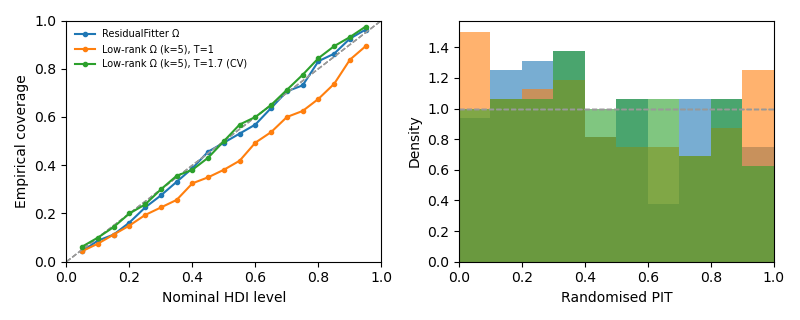
Left: fraction of trials whose q-HDI contains the true stimulus (diagonal = calibrated). Right: randomised PIT (flat = calibrated).
The model
\(D\) — per-voxel residual SD (times one overall ML scale factor);
\(F\) — the first
kprincipal factors of the residual correlation matrix (eigenvectors × √eigenvalues; one closed-form principal-factor step);\(\Psi\) — diagonal uniquenesses \(1 - \mathrm{diag}(F F^\top)\), floored at
psi_floor(default 0.02).
The likelihood is multivariate Student-t (ν by maximum likelihood, a 1-D
search with the scale profiled out by EM) or Gaussian (dof=None). Ω is
never formed as a dense matrix: the Mahalanobis distance uses the
Woodbury identity and the log-determinant the matrix-determinant lemma,
so evaluating the likelihood costs \(O(Vk)\) per residual vector. For a
grid of candidate stimuli, data and grid predictions are projected once
and the whole (trials × stimuli) table is one matrix product. Both are
float64 numpy; LowRankNoise.log_prob_backend() gives the same
log-density in Keras ops (TF / JAX / torch, differentiable) for use inside
a gradient-based stimulus fitter.
The posterior is tempered:
T > 1 widens the posterior without moving its mode; T = ∞ is a flat
posterior. get_stimulus_pdf applies the noise model’s temperature,
or any temperature= you pass (also with a dense omega=).
Choosing k and T by nested cross-validation
LowRankNoise.fit splits the training trials by groups (runs).
For each held-out group g and each candidate k:
Ω(k) and ν are fitted on the residuals of the other groups;
the held-out trials are decoded on the grid, giving a log-likelihood table;
for every candidate T, the log posterior probability of the true stimulus, \(\log p_T(s^* \mid y)\), is summed over trials.
The (k, T) with the highest total over all held-out groups is chosen and
Ω is refitted on all training trials with that k. noise.cv_scores_
holds the full table (mean nats per trial relative to a flat posterior).
Defaults: k ∈ {0, 1, 2, 5, 10, 20, 40, 80} (capped by the number of
inner-training trials and voxels), T ∈ {2^-2, …, 2^12} in steps of
2^¼ plus ∞. Pass k=40 and/or temperature=2.0 to fix either.
The criterion is the decoding objective, not the covariance likelihood. On 7T single-trial betas the held-out covariance likelihood keeps improving up to k = 160 while decoding gets worse beyond k ≈ 40; choosing k by covariance fit would pick the wrong model.
The best k is data-dependent, which is why it is cross-validated rather
than fixed. In a 19-participant validation on the same data (two ROIs ×
16 leave-one-run-out folds, smoothed betas, ~2,000 voxels, 480 training
trials), the nested CV chose k = 0 — a diagonal Student-t with
per-voxel scales and no shared factors — in ~60% of folds and k = 10 in
~17%, with T ≈ 360 (median). That beat both the production Ω and a fixed
k = 40 with CV-chosen T on held-out log score, and gave 95% joint HDI
coverage of 0.94 (production: 0.79). Always report the chosen k and T
(noise.summary()).
Encoding parameters inside the inner folds (inner_parameters):
None(default) — the parameters you pass are held fixed. The inner held-out trials were then part of the data the encoding model was fitted to, so their predictions are a little optimistic and T may come out slightly too small.a
dict{group: parameters}of parameters that did not see group g (e.g. existing leave-one-run-out fits), ora callable
f(train_data, train_paradigm, group) -> parametersthat refits the encoding model on the inner-training trials (cleanest, slowest).
Why not ResidualFitter’s Ω?
On 7T single-trial numerosity betas (19 participants; see the
retinonumeral project notes) three problems were found:
The one-factor Ω underestimates held-out noise.
ResidualFittermodels \(\rho\,\tau\tau^\top + (1-\rho)\,\mathrm{diag}(\tau^2) + \sigma^2 WW^\top\): one shared factor. Real residuals need tens of factors (5 PCs ≈ 70% of the variance, 20 PCs ≈ 90%). Held-out squared Mahalanobis distances were ~4× larger than Ω implies, ~16× along the decoding directions, and every participant’s posteriors scored worse than a flat one (95% HDI coverage 0.79).``lambd`` shrinkage is unsafe when voxels > trials. Mixing in the sample covariance of n < V trials leaves near-null directions in which held-out residuals explode (coverage ≈ 0.04 at
lambd=0.5).The pseudo-WWᵀ is uncentred.
init_pseudoWWTbuilds WWᵀ from raw (uncentred, mean-normalised) predicted responses, so it is dominated by the common-mode response rather than by the directions that discriminate stimuli.
A low-rank Ω alone makes posteriors sharper — and at T = 1 even more overconfident — but it whitens away shared noise and roughly doubled the correlation between posterior mean and true stimulus in a 4-participant pilot (in the 19-participant validation, CV-chosen k and T raised it from 0.05 to 0.14). The CV temperature (there T ≈ 60–600, reflecting how little calibrated information there is about the stimulus) then brings coverage to nominal. Use both.
Legacy / functional path
Code that passes dense omega= / dof= can use:
from braincoder.noise import fit_lowrank_omega
omega, dof = fit_lowrank_omega(residuals, k=40)
pdf = model.get_stimulus_pdf(test_data, grid, omega=omega, dof=dof,
                             temperature=T)
or noise.to_dense(). ResidualFitter and the default behaviour of
get_stimulus_pdf are unchanged.
API
Full reference: Noise models for decoding and Calibration diagnostics in the API Reference.