Geodesic-regularised noise model for trial-wise decoding

For Bayesian decoding from an encoding model, the noise covariance \(\Omega\) between voxels matters as much as the tuning curves themselves. The simplest assumption is uncorrelated isotropic noise (diagonal \(\Omega\)), but real fMRI noise has substantial spatially-structured correlations — voxels that sit near each other on the cortical sheet share more noise than distant ones.

braincoder’s braincoder.optimize.ResidualFitter lets you parameterise this directly. With D=None (default) it fits a model where covariance is driven only by tuning similarity (\(\tau\tau^T\)) plus an isotropic component. With D=<pairwise distance matrix> it adds a distance-modulated component:

\[\Omega = \rho\,\bigl[\alpha \cdot (e^{-\beta D} \odot \tau\tau^T) + (1 - \alpha) \cdot \tau\tau^T \bigr] + (1 - \rho)\,\mathrm{diag}(\tau^2) + \sigma^2 W W^T\]

where \(D\) is voxel-to-voxel distance, and \(\alpha,\beta\) are learned from data. Plug in geodesic distance on the cortical mesh (rather than Euclidean) and you respect the fact that two voxels sitting on opposite banks of a sulcus are close in 3D but functionally far apart.

This example fits a numerosity tuning model in right parietal cortex (NPCr), then compares decoding with isotropic-ish vs. geodesic-regularised \(\Omega\).

import matplotlib.pyplot as plt
import numpy as np
import pandas as pd

from braincoder.models import LogGaussianPRF
from braincoder.optimize import ParameterFitter, ResidualFitter
from braincoder.utils.cortex import geodesic_distance_matrix
from braincoder.utils.data import load_pratcarrabin2025_npc
from braincoder.utils.stats import (
    fit_r2_mixture,
    get_rsq,
)

Load the demo bundle and select responsive voxels

We re-run the same mixture-model selection from example 1 so the notebooks are independent. We then keep only voxels with \(P(\\text{signal} \\mid r^2) \\ge 0.8\) and restrict to one stimulus range (wide) to keep the model simple.

bundle = load_pratcarrabin2025_npc()
r2 = bundle['r2']
paradigm_all = bundle['paradigm']
data_all = bundle['data']

r2_wb = bundle['r2_wholebrain'].get_fdata()
mask_wb = bundle['brain_mask'].get_fdata().astype(bool)
fit = fit_r2_mixture(r2_wb[mask_wb])
# Noise μ + 2σ on the logit scale — see example 1 for the rationale.
threshold = 1.0 / (1.0 + np.exp(-(fit['noise_mu'] + 2 * fit['noise_sigma'])))
keep = r2.index[r2 > threshold]
print(f'Kept {len(keep)}/{len(r2)} voxels (within-sample R² ≥ {threshold:.3f})')

is_wide = paradigm_all['range'].values == 'wide'
paradigm = paradigm_all.loc[is_wide].reset_index(drop=True)
data = data_all.loc[is_wide, keep].reset_index(drop=True)
data = data.astype(np.float32)
# Per-voxel z-score within the kept set so the model only sees signal scale.
data = (data - data.mean(axis=0)) / data.std(axis=0).replace(0, 1)
print(f'Data: {data.shape}  (trials × voxels)')

Kept 155/852 voxels (within-sample R² ≥ 0.085)
Data: (240, 155)  (trials × voxels)

Fit a Log-Gaussian PRF per voxel

The encoding model has 4 parameters per voxel — mu (preferred numerosity), sd (tuning width), amplitude, baseline.

stim = paradigm[['n']].astype(np.float32).values

model = LogGaussianPRF(parameterisation='mu_sd_natural')

n_train = int(0.75 * len(stim))
train_idx = np.arange(n_train)
test_idx = np.arange(n_train, len(stim))

fitter = ParameterFitter(model, data.iloc[train_idx],
                          paradigm[['n']].iloc[train_idx])
init = pd.DataFrame({
    'mu':        np.full(data.shape[1], 25.0),
    'sd':        np.full(data.shape[1], 10.0),
    'amplitude': np.full(data.shape[1], 1.0),
    'baseline':  np.full(data.shape[1], 0.0),
}, index=data.columns, dtype=np.float32)

# Coarse grid-init helps the optimiser find a decent starting mu.
mu_grid = np.linspace(10, 40, 16, dtype=np.float32)
sd_grid = np.array([5., 10., 20.], dtype=np.float32)
amp_grid = np.array([0.5, 1.0, 2.0], dtype=np.float32)
base_grid = np.array([0.0], dtype=np.float32)
init = fitter.fit_grid(mu_grid, sd_grid, amp_grid, base_grid)

pars = fitter.fit(max_n_iterations=600, init_pars=init,
                   noise_model='gaussian', learning_rate=0.05,
                   progressbar=False)
train_pred = model.predict(paradigm=paradigm[['n']].iloc[train_idx],
                            parameters=pars)
train_pred.index = data.iloc[train_idx].index
train_r2 = get_rsq(data.iloc[train_idx], train_pred)
print(f'Train R² — median {np.nanmedian(train_r2):.3f}, '
      f'p90 {np.nanpercentile(train_r2, 90):.3f}')

Working with chunk size of 23894

  0%|          | 0/1 [00:00<?, ?it/s]
100%|██████████| 1/1 [00:00<00:00, 38.27it/s]
Number of problematic voxels (mask): 0
Number of voxels remaining (mask): 155
*** Fitting: ***
 * mu
 * sd
 * amplitude
 * baseline
Train R² — median 0.115, p90 0.174

Build the geodesic distance matrix

The demo bundle ships a cropped cortical-mesh patch (right hemisphere white-matter surface), plus a per-voxel “nearest patch vertex” index. geodesic_distance_matrix runs Dijkstra along mesh edges and returns the pairwise distance between only the seed vertices we ask for.

voxel_to_vertex = bundle['voxel_to_vertex'].loc[keep, 'vertex'].values
D = geodesic_distance_matrix(
    bundle['surface_vertices'],
    bundle['surface_faces'],
    source_indices=voxel_to_vertex,
    progressbar=False,
)
print(f'Distance matrix: {D.shape}, '
      f'median pairwise distance {np.median(D[np.triu_indices_from(D, k=1)]):.1f} mm')

Distance matrix: (155, 155), median pairwise distance 32.9 mm

Fit two noise models

Each ResidualFitter is fit to the same residuals; the only difference is whether we pass the geodesic distance matrix.

resid = data.iloc[train_idx].values - train_pred.values
resid_df = pd.DataFrame(resid, columns=data.columns)

# ``ResidualFitter`` needs a ``W Wᵀ`` template covariance that summarises
# how voxel responses co-vary across the stimulus range. We compute it
# once over a dense stimulus grid and reuse it for both fits below.
stim_grid_fit = pd.DataFrame({'n': np.linspace(10, 40, 31)})
stim_grid_fit.index.name = 'stimulus'
model.init_pseudoWWT(stim_grid_fit, pars)

print('Fitting Ω without distance regularisation …')
rf_std = ResidualFitter(model, data.iloc[train_idx],
                         paradigm[['n']].iloc[train_idx],
                         parameters=pars)
omega_std, dof_std = rf_std.fit(method='t', init_dof=10.0,
                                  max_n_iterations=400, progressbar=False)

print('Fitting Ω with geodesic-distance regularisation …')
rf_geo = ResidualFitter(model, data.iloc[train_idx],
                         paradigm[['n']].iloc[train_idx],
                         parameters=pars)
omega_geo, dof_geo = rf_geo.fit(method='t', init_dof=10.0,
                                  D=D, init_alpha=0.5, init_beta=0.05,
                                  max_n_iterations=400, progressbar=False)
print(f'  fitted dof:  std={dof_std:.1f}, geo={dof_geo:.1f}')
print(f'  fitted α/β:  α={rf_geo.fitted_omega_parameters["alpha"]:.2f}, '
      f'β={float(rf_geo.fitted_omega_parameters["beta"]):.3f}')

Fitting Ω without distance regularisation …
init_tau: 0.8757237792015076, 1.0135356187820435
USING A PSEUDO-WWT!
WWT max: 69.62195587158203
Fitting Ω with geodesic-distance regularisation …
init_tau: 0.8757237792015076, 1.0135356187820435
USING A PSEUDO-WWT!
WWT max: 69.62195587158203
  fitted dof:  std=6.8, geo=10.8
  fitted α/β:  α=0.93, β=0.088

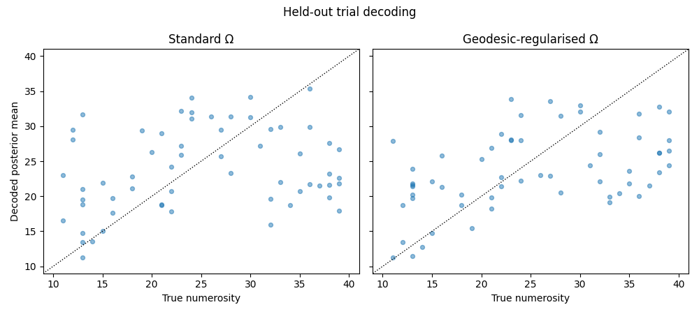
Decode the held-out trials with each Ω

model.get_stimulus_pdf returns the posterior \(P(s \\mid y)\) over a stimulus grid, given the data, fitted parameters, and noise model. We compute it for each held-out trial under both Ωs and compare the posterior means.

stim_grid = pd.DataFrame({'n': np.linspace(10, 40, 60)})
stim_grid.index.name = 'stimulus'

post_std = model.get_stimulus_pdf(
    data.iloc[test_idx], parameters=pars, stimulus_range=stim_grid,
    omega=omega_std, dof=dof_std)
post_geo = model.get_stimulus_pdf(
    data.iloc[test_idx], parameters=pars, stimulus_range=stim_grid,
    omega=omega_geo, dof=dof_geo)

def posterior_mean_and_sd(post, grid):
    s = grid['n'].values
    p = post.values / post.values.sum(axis=1, keepdims=True)
    mean = (p * s).sum(axis=1)
    var  = (p * (s[None, :] - mean[:, None]) ** 2).sum(axis=1)
    return mean, np.sqrt(var)

mu_std, sd_std = posterior_mean_and_sd(post_std, stim_grid)
mu_geo, sd_geo = posterior_mean_and_sd(post_geo, stim_grid)
true_n = paradigm['n'].iloc[test_idx].values

err_std = mu_std - true_n
err_geo = mu_geo - true_n
print(f'Test posterior-mean RMSE  std: {np.sqrt(np.mean(err_std**2)):.2f}, '
      f'geo: {np.sqrt(np.mean(err_geo**2)):.2f}')

Test posterior-mean RMSE  std: 9.69, geo: 8.32

Visualise

fig, axes = plt.subplots(1, 2, figsize=(10, 4.5), sharey=True)
for ax, mu_post, label in [(axes[0], mu_std, 'Standard Ω'),
                             (axes[1], mu_geo, 'Geodesic-regularised Ω')]:
    ax.scatter(true_n, mu_post, alpha=0.5, s=18, color='#1f77b4')
    lim = (true_n.min() - 2, true_n.max() + 2)
    ax.plot(lim, lim, 'k:', lw=1)
    ax.set_xlim(lim); ax.set_ylim(lim)
    ax.set_xlabel('True numerosity')
    ax.set_title(label)
axes[0].set_ylabel('Decoded posterior mean')
fig.suptitle('Held-out trial decoding')
plt.tight_layout()
plt.show()

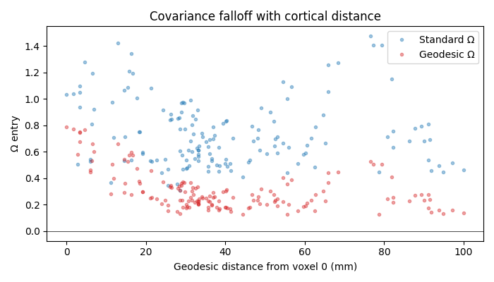
Inspect Ω structure

Sort voxels by their geodesic distance to a seed voxel and look at the implied covariance row. The geodesic-regularised \(\\Omega\) should drop off smoothly with distance, while the standard fit can show high correlations regardless of distance.

seed = 0
order = np.argsort(D[seed])

fig, ax = plt.subplots(figsize=(7, 4))
ax.plot(D[seed, order], omega_std[seed, order], '.', alpha=0.4,
         label='Standard Ω')
ax.plot(D[seed, order], omega_geo[seed, order], '.', alpha=0.4,
         label='Geodesic Ω', color='#d62728')
ax.axhline(0, color='k', lw=0.5)
ax.set_xlabel(f'Geodesic distance from voxel {seed} (mm)')
ax.set_ylabel('Ω entry')
ax.set_title('Covariance falloff with cortical distance')
ax.legend()
plt.tight_layout()
plt.show()