Lesson 2: Linear encoding models

A linear encoding approach

In the previous lesson, we saw how we can define (non-linear) encoding models and fit their parameter \(\theta\) to predict voxel responses \(x\) using non-linear descent.

It is important to point out that in most of the literature, the parameters \(\theta\) are asssumed to be fixed. In such work, researchers assume a limited set of \(m\) neural populations, each with their own set of parameters \(\theta\).

The responses in different \(n\) neural measures (e.g., fMRI voxels) are then to assume to be a linear combination of these fixed neural populations. How much each neural population contributes to each voxel is then defined by a weight matrix \(W\) of size \(m \times n\).

\[x_j = \sum W_{i, j} \cdot f_j(\theta_j)\]

The big advantage of this approach is that it allows us fit the weight matrix \(W\) using linear regression. This is a much, much faster approach than fitting the parameters \(\theta\) using non-linear gradient descent.

In this lesson, we will see how we can use the EncodingModel class to fit linear encoding models.

Setting up a linear encoding model in braincoder

In braincoder, we can set up a linear encoding model by defining a fixed number of neural encoding populations, each with their own parameters set \(\theta_j\).

Here we use a Von Mises tuning curve to define the neural populations that are senstive to the orientation of a grating stimulus. Note that orientations are given in radians, so lie between -pi and pi.

Set up a von Mises model

from braincoder.models import VonMisesPRF
import numpy as np
import pandas as pd
import matplotlib.pyplot as plt

# Set up six evenly spaced von Mises PRFs
centers = np.linspace(0.0, 2*np.pi, 6, endpoint=False)
parameters = pd.DataFrame({'mu':centers, 'kappa':1., 'amplitude':1.0, 'baseline':0.0},
                          index=pd.Index([f'Voxel {i+1}' for i in range(6)], name='voxel'))

# We have 3 voxels, each with a linear combination of the 6 von Mises functions:
weights = np.array([[1, 0, 1],
                    [1, .5, 1],
                    [0, 1, 0],
                    [0, .5, 0],
                    [0, 0, 1],
                    [0, 0, 1]]).astype(np.float32)

model = VonMisesPRF(parameters=parameters, weights=weights)

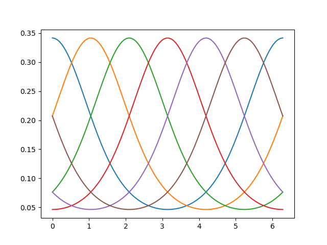
Once we have set up the model, we can first have a look at the predictions for the 6 different basis functions:

# Note that the function `basis_functions` returns a `tensorflow` `Tensor`,
# which has to be converted to a numpy array:
orientations = np.linspace(0, np.pi*2, 100)
basis_responses = model.basis_predictions(orientations, parameters).numpy()

_ = plt.plot(orientations, basis_responses)

Because the model also has a \(n{\times}m\) weight matrix (number of voxels x number of neural populations), we can also use the model to predict the responses of different voxels to the same orientation stimuli:

# Each voxel timeseries is a weighted sum of the six basis functions
pred = model.predict(paradigm=orientations)
_ = plt.plot(orientations, pred)

Fit a linear encoding model using (regularised) OLS

To fit linear encoding models we can use the braincoder.optimize.WeightFitter. This fits weights to the model using linear regression. Note that one can also provide an alpha-parameter to the WeightFitter to regularize the weights (pull them to 0; equivalent to putting a Gaussian prior on the weights). This is often a very good idea in real data!

from braincoder.optimize import WeightFitter
from braincoder.utils import get_rsq

# Simulate data
data = model.simulate(paradigm=orientations, noise=0.1)

# Fit the weights
weight_fitter = WeightFitter(model, parameters, data, orientations)
estimated_weights = weight_fitter.fit(alpha=0.1)

# Get predictions for the fitted weights
pred = model.predict(paradigm=orientations, weights=estimated_weights)
r2 = get_rsq(data, pred)

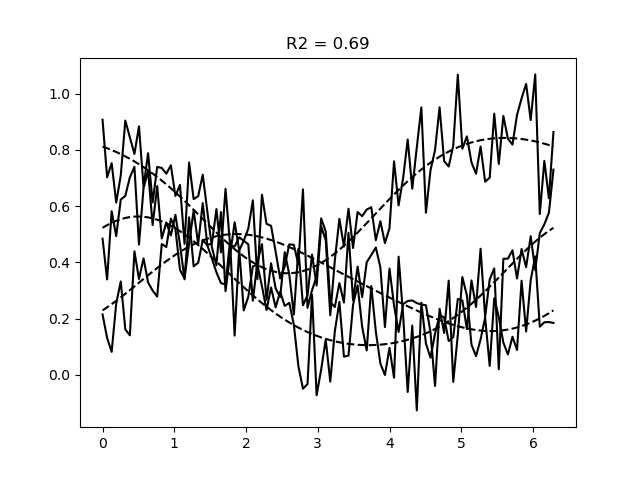
# Plot the data and the predictions
plt.figure()
plt.plot(orientations, data, c='k')
plt.plot(orientations, pred.values, c='k', ls='--')
plt.title(f'R2 = {r2.mean():.2f}')

Note

The complete Python script and its output can be found here.

Summary

In this lesson, we had a look at linear encoding models. These models:

• Assume a fixed number of neural populations, each with their own parameters \(\theta_j\)

• Every voxel then is assumed to be a linear combination of these neural populations

• The weights of this linear combination can be fit using linear regression

• This is much faster than fitting the parameters \(\theta_j\) using non-linear gradient descent

In the next lesson, we will see how we can add a noise model to the encoding models, which yields a likelihood function which we can invert in a principled manner.