Voxel selection via a 2-component R² mixture model

When you fit an encoding model to whole-brain fMRI data, most voxels are genuinely noise — they don’t tune to the stimulus dimension you’re modelling. Almost every downstream analysis (decoding, Fisher information, expected uncertainty) needs a way to select voxels that actually carry signal, without hand-picking an arbitrary R² cutoff.

A simple data-driven approach is to fit a 2-component Gaussian mixture on logit(R²). One component captures the bulk of noise voxels, the other the tail of well-tuned voxels. From the fitted mixture you can derive a threshold in several ways:

• Posterior-based — keep voxels with \(P(\text{signal} \mid r^2) \ge p\). Smooth, but the effective cap depends on how separable the two components are.

• Tail-FDR — keep voxels where the false-discovery rate of the noise component crossing the threshold is below \(\alpha\). Classical, works cleanly when the two modes are well separated.

• Noise-tail quantile — keep voxels with R² above the noise component’s \(\mu_n + k\sigma_n\) on the logit scale. A conservative “R² unlikely under noise alone” criterion that produces selective masks even when the two mixture modes overlap heavily.

This example walks through the three options on a real subject’s whole-brain within-sample R², then applies the chosen threshold inside the NPCr ROI to derive the voxel mask used by the rest of the pipeline.

The demo data is a small bundle (~4 MB) extracted from one subject of the numerosity fMRI dataset in Prat-Carrabin et al. (2025, bioRxiv 10.1101/2025.09.25.675916); it’s downloaded automatically on first run.

import matplotlib.pyplot as plt
import numpy as np
import pandas as pd

from braincoder.utils.data import load_pratcarrabin2025_npc
from braincoder.utils.stats import (
    fit_r2_mixture,
    r2_fdr_threshold,
    r2_p_signal_threshold,
    plot_r2_mixture,
)

Load the demo bundle

load_pratcarrabin2025_npc returns a dict with both whole-brain and NPCr-only data. For voxel selection we use the whole-brain within-sample R² — the fraction of variance the encoding model explains on the data it was fit to. That quantity is bounded in \([0, 1]\), so every brain voxel contributes to the mixture. CV-R² is the right tool for reporting generalisation, but it can go arbitrarily negative when a model overfits — and the mixture loses half its data if you drop those voxels.

bundle = load_pratcarrabin2025_npc()
print('Subject:', bundle['manifest']['subject'])

r2_img     = bundle['r2_wholebrain']         # nibabel Nifti1Image
brain_mask = bundle['brain_mask']            # nibabel Nifti1Image, T1w
r2_npcr    = bundle['r2']                    # NPCr-only R² (pd.Series)
cvr2_npcr  = bundle['cv_r2']                 # NPCr-only CV-R² (for sanity)

r2_wb = r2_img.get_fdata()
mask_wb = brain_mask.get_fdata().astype(bool)
r2_in_brain = r2_wb[mask_wb]
r2_in_brain = r2_in_brain[np.isfinite(r2_in_brain)]

print(f'In-brain voxels: {len(r2_in_brain):,}')
print(f'  R²>0:    {(r2_in_brain > 0).sum():,}')
print(f'  R²>0.05: {(r2_in_brain > 0.05).sum():,}')
print(f'  R²>0.10: {(r2_in_brain > 0.10).sum():,}')

Subject: sub-13
In-brain voxels: 72,438
  R²>0:    70,201
  R²>0.05: 5,537
  R²>0.10: 1,133

Fit the mixture

fit_r2_mixture internally filters to 0 < R² < 0.99 and fits a 2-component Gaussian mixture on the logit-transformed values. The return is a dictionary describing both components and the fit.

fit = fit_r2_mixture(r2_in_brain)
print(f"Noise:  mean R²={fit['noise_mean_r2']:.4f},  "
      f"weight={fit['noise_weight']:.2f}")
print(f"Signal: mean R²={fit['signal_mean_r2']:.4f},  "
      f"weight={fit['signal_weight']:.2f}")

Noise:  mean R²=0.0023,  weight=0.32
Signal: mean R²=0.0117,  weight=0.68

Derive thresholds

Compute thresholds three ways. For this dataset the signal mode isn’t strongly separated from noise, so the posterior-based threshold caps out somewhere around \(P \\approx 0.85\) and tail-FDR only converges at permissive \(\\alpha\). The noise-tail quantile still gives a useful selective cutoff in that regime.

post_thresholds = {
    p: r2_p_signal_threshold(fit, p=p) for p in [0.5, 0.7, 0.8, 0.85]
}
fdr_thresholds = {
    a: r2_fdr_threshold(fit, alpha=a) for a in [0.05, 0.10, 0.20]
}
# Noise-tail cutoff: invert logit at noise_mu + k*noise_sigma.
def _inv_logit(z):
    return 1.0 / (1.0 + np.exp(-z))
noise_tail_thresholds = {
    k: _inv_logit(fit['noise_mu'] + k * fit['noise_sigma'])
    for k in [1, 2, 3]
}

print('\nPosterior P(signal | R²) thresholds:')
for p, thr in post_thresholds.items():
    txt = f'{thr:.4f}' if np.isfinite(thr) else '∞ (degenerate)'
    print(f'   P≥{p:.2f}   →  R² ≥ {txt}')

print('\nTail-FDR thresholds:')
for a, thr in fdr_thresholds.items():
    txt = f'{thr:.4f}' if np.isfinite(thr) else '∞ (degenerate)'
    print(f'   α={a:.2f}    →  R² ≥ {txt}')

print('\nNoise-tail (R² unlikely under noise component):')
for k, thr in noise_tail_thresholds.items():
    print(f'   μ_n + {k}σ_n →  R² ≥ {thr:.4f}')

# We use the **noise μ + 2σ** cutoff as the operating point. On the
# logit scale that's roughly the 97.5th percentile of the noise
# component — i.e. an R² above this is unlikely to come from a
# pure-noise voxel.
threshold = noise_tail_thresholds[2]
print(f'\nChosen threshold (noise μ+2σ): R² ≥ {threshold:.4f}')

Posterior P(signal | R²) thresholds:
   P≥0.50   →  R² ≥ 0.0020
   P≥0.70   →  R² ≥ 0.0040
   P≥0.80   →  R² ≥ 0.0073
   P≥0.85   →  R² ≥ 0.0134

Tail-FDR thresholds:
   α=0.05    →  R² ≥ ∞ (degenerate)
   α=0.10    →  R² ≥ ∞ (degenerate)
   α=0.20    →  R² ≥ 0.0023

Noise-tail (R² unlikely under noise component):
   μ_n + 1σ_n →  R² ≥ 0.0145
   μ_n + 2σ_n →  R² ≥ 0.0847
   μ_n + 3σ_n →  R² ≥ 0.3674

Chosen threshold (noise μ+2σ): R² ≥ 0.0847

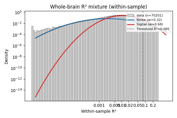
Diagnostic plot

plot_r2_mixture overlays the histogram of logit(R²), the two fitted component densities, and the chosen threshold (x-ticks are labelled on the raw R² scale).

fig = plot_r2_mixture(fit, r2=r2_in_brain, threshold=threshold,
                      title='Whole-brain R² mixture (within-sample)')
fig.axes[0].set_xlabel('Within-sample R²')
plt.tight_layout()
plt.show()

Apply the threshold inside NPCr

The threshold was learned on the whole brain (where there are plenty of genuine-noise voxels to anchor the noise component). We then apply it to the NPCr within-sample R² to derive the voxel mask used by the decoder and uncertainty notebooks. The kept voxels are the ones whose tuning curves the encoding model was able to explain; their CV-R² (right-hand plot) shows how that signal transfers to unseen trials.

n_npcr = len(r2_npcr)
keep = r2_npcr > threshold
print(f'NPCr voxels: {n_npcr},  passing threshold: {int(keep.sum())} '
      f'({100 * keep.mean():.1f}%)')

fig, axes = plt.subplots(1, 2, figsize=(11, 4), sharey=True)
ax = axes[0]
ax.hist(r2_npcr, bins=40, color='0.7', edgecolor='0.4',
        label=f'All NPCr (n={n_npcr})')
ax.hist(r2_npcr[keep], bins=40, color='#d62728', alpha=0.8,
        label=f'Kept (n={int(keep.sum())})')
ax.axvline(threshold, color='k', ls='--', lw=1,
           label=f'R²≥{threshold:.3f}')
ax.set_xlabel('Within-sample R² (NPCr)')
ax.set_ylabel('Number of voxels')
ax.set_title('Selection')
ax.legend()

ax = axes[1]
ax.hist(cvr2_npcr, bins=40, color='0.7', edgecolor='0.4',
        label='All NPCr')
ax.hist(cvr2_npcr[keep], bins=40, color='#d62728', alpha=0.8,
        label='Kept (by within-sample R²)')
ax.axvline(0, color='k', lw=0.6)
ax.set_xlabel('Cross-validated R² (NPCr)')
ax.set_title('Generalisation of the kept set')
ax.legend()

plt.tight_layout()
plt.show()

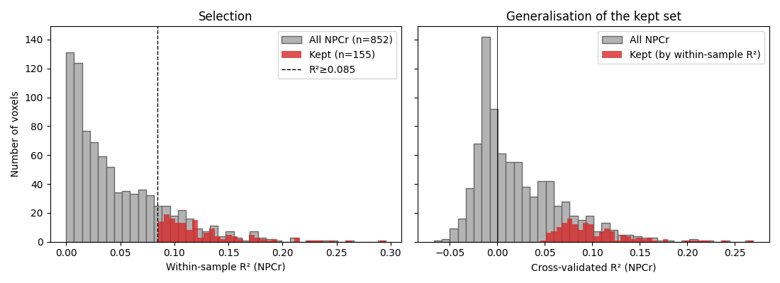
NPCr voxels: 852,  passing threshold: 155 (18.2%)

Save the mask for the next notebook

The decoder and expected-uncertainty examples both start from this same mask. We don’t actually persist it here — they refit the mixture for self-contained reproducibility — but in your own pipeline you’d typically pickle / write a TSV with the selected voxel ids:

keep_ids = cvr2_npcr.index[keep]
pd.Series(keep_ids).to_csv('selected_voxels.tsv', index=False)