Decoding 2D stimuli from neural data

Here, we are decoding oriented stimuli from neural data that have an extra dimension: amplitude.

Amplitude can be interpreted as the stimulus drive and has been shown to be modulated by cognitive effects such as expectation and attention.

# Set up a neural model
from braincoder.models import VonMisesPRF
import numpy as np
import pandas as pd
import scipy.stats as ss
noise = 0.5

# We are setting up a VonMisesPRF model with 8 orientations,
# We have 8 voxels, each with a linear combination of the 8 von Mises functions
# We use the identity matrix with some noice, so that each voxel is driven by
# largely by a single PRF
parameters = pd.DataFrame({'mu':np.linspace(0, 2*np.pi, 8, False), 'kappa':1.0, 'amplitude':1.0, 'baseline':0.0})

weights = np.identity(8) * 5.0
weights += np.random.rand(8, 8)
model = VonMisesPRF(parameters=parameters, model_stimulus_amplitude=True, weights=weights)

# Note how the stimulus type is now `OneDimensionalRadialStimulusWithAmplitude`
# which means that the stimulus is two-dimensional
print(model.stimulus)
print(model.stimulus.dimension_labels)

<braincoder.stimuli.OneDimensionalRadialStimulusWithAmplitude object at 0x179935250>
['x (radians)', 'amplitude']

# Now we can simulate some data and estimate parameters+noise
mapper_paradigm = pd.DataFrame({'x (radians)':np.random.rand(100)*2*np.pi, 'amplitude':1.})
data = model.simulate(paradigm=mapper_paradigm, noise=noise)

# Set up parameter fitter
from braincoder.optimize import WeightFitter, ResidualFitter
fitter = WeightFitter(model, parameters, data, mapper_paradigm)
# With 8 overlapping Von Mises functions, we already need some regularisation, hence alpha=1.0
fitted_weights = fitter.fit(alpha=1.0)

# Now we fit the covariance matrix on the residuals
resid_fitter = ResidualFitter(model, data, mapper_paradigm, parameters, fitted_weights)
omega, dof = resid_fitter.fit(progressbar=False)

init_tau: 0.4727478325366974, 0.5595152378082275
WWT max: 15.28452205657959

# Now we set up an experimental paradigm with two conditions
# An `attended` and an `unattended` condition.
# In the attended condition, the stimulus will have more drive (1.5),
# in the unattended condition, the stimulus will have less drive (0.5).

n = 200
experimental_paradigm = pd.DataFrame(index=pd.MultiIndex.from_product([np.arange(n/2.), ['attended', 'unattended']], names=['frame', 'condition']))

# Random orientations
experimental_paradigm['x (radians)'] = np.random.rand(n)*2*np.pi

# Amplitudes have some noise
experimental_paradigm['amplitude'] = np.where(experimental_paradigm.index.get_level_values('condition') == 'attended', ss.norm(1.5, 0.1).rvs(n), ss.norm(.5, 0.1).rvs(n))
experimental_data = model.simulate(paradigm=experimental_paradigm, noise=noise)
# Restore the MultiIndex (simulate() flattens it to a single 'stimulus' level)
experimental_data.index = experimental_paradigm.index

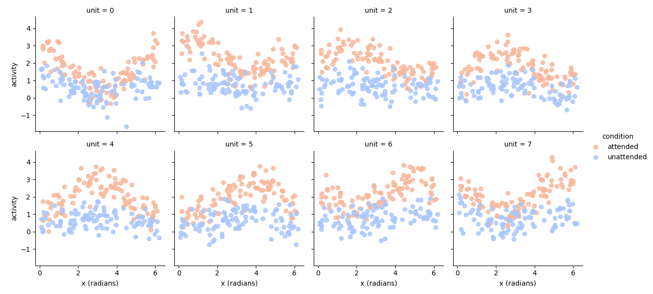
# Plot the data
import seaborn as sns
import matplotlib.pyplot as plt
tmp = experimental_data.set_index(experimental_paradigm['x (radians)'], append=True).stack().to_frame('activity')
g = sns.FacetGrid(tmp.reset_index(), col='unit', col_wrap=4, hue='condition', palette='coolwarm_r')
g.map(plt.scatter, 'x (radians)', 'activity', alpha=0.85)
g.add_legend()

<seaborn.axisgrid.FacetGrid object at 0x17992e870>

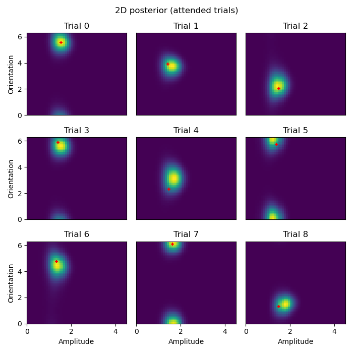
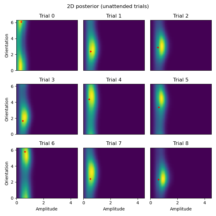
# Now we can calculate the 2D likelihood/posterior of different orientations+amplitudes for the data
lower_amplitude, higher_amplitude = 0.0, 4.5
potential_amplitudes = np.linspace(lower_amplitude, higher_amplitude, 50)
potential_orientations = np.linspace(0, 2*np.pi, 50, False)

# Make sure ground truth is the potential stimuli
potential_amplitudes = np.sort(np.append(potential_amplitudes, [0.5, 1.5]))

# We use the `pd.MultiIndex.from_product` function to create a grid of possible stimuli
potential_stimuli = pd.MultiIndex.from_product([potential_orientations, potential_amplitudes], names=['x (radians)', 'amplitude']).to_frame(index=False)

# Now we get, for each data point, the likelihood of each possible stimulus
ll = model.get_stimulus_pdf(experimental_data, potential_stimuli, omega=omega, dof=dof,
                            include_multidimensional_stimulus_index=True)

# Plot 2D posteriors for first 9 trials

# Once we have these 2D likelihoods, now we want to be able to plot them.
def plot_trial(key, ll=ll, paradigm=experimental_paradigm, xlabel=False, ylabel=False):
    # We use the `stack` method to turn the `amplitude` dimension into a column
    ll = ll.loc[key].unstack('amplitude')

    # Use imshow to show a 2D image of the likelihood
    vmin, vmax = ll.min().min(), ll.max().max()
    plt.imshow(ll, origin='lower', aspect='auto', extent=[lower_amplitude, higher_amplitude, 0, 2*np.pi], vmin=vmin, vmax=vmax)

    # Plot the _actual_ ground truth amplitude and orientation
    plt.scatter(paradigm.loc[key]['amplitude'], paradigm.loc[key]['x (radians)'], c='r', s=25, marker='+')

    # Some housekeeping for the subplots
    plt.title(f'Trial {key[0]}')
    if xlabel:
        plt.xticks()
        plt.xlabel('Amplitude')
    else:
        plt.xticks([])

    if ylabel:
        plt.yticks()
        plt.ylabel('Orientation')
    else:
        plt.yticks([])

def plot_condition(condition):
    """
    Plot the 2D posterior for a given condition for the first 9 trials.

    Parameters:
    condition (str): The condition for which to plot the posterior.

    Returns:
    None
    """
    plt.figure(figsize=(7, 7))
    for ix in range(9):
        plt.subplot(3, 3, ix+1)

        xlabel = ix in [6, 7, 8]
        ylabel = ix in [0, 3, 6]

        plot_trial((ix, condition), xlabel=xlabel, ylabel=ylabel)

    plt.suptitle(f'2D posterior ({condition} trials)')
    plt.tight_layout()

plot_condition('attended')
plot_condition('unattended')

• 
• 

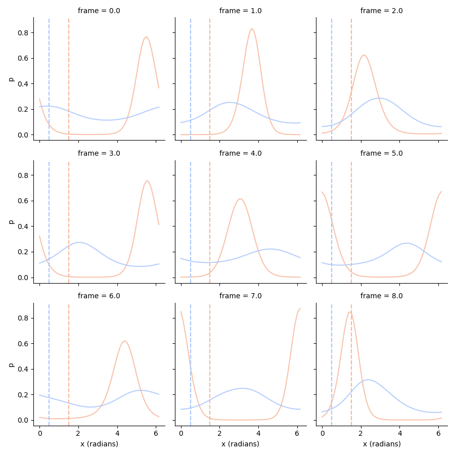
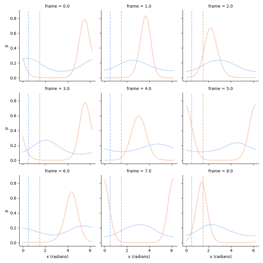
# Now we can calculate the 1D posterior for specific orientations _or_ amplitudes

# Marginalize out orientations
amplitudes_posterior = ll.T.groupby(level='amplitude').sum().T
amplitudes_posterior = amplitudes_posterior.div(np.trapezoid(amplitudes_posterior, amplitudes_posterior.columns, axis=1), axis=0) # This is the same as normalizing the posterior

# Marginalize out amplitudes
orientations_posterior = ll.T.groupby(level='x (radians)').sum().T
orientations_posterior = orientations_posterior.div(np.trapezoid(orientations_posterior, orientations_posterior.columns, axis=1), axis=0)

# Plot orientation posteriors
tmp = orientations_posterior.stack().loc[:8].to_frame('p')

g = sns.FacetGrid(tmp.reset_index(), col='frame', col_wrap=3, hue='condition', palette='coolwarm_r')
g.map(plt.plot, 'x (radians)', 'p', alpha=0.85)

g.map(plt.axvline, x=1.5, c=sns.color_palette('coolwarm_r', 2)[0], ls='--')
g.map(plt.axvline, x=0.5, c=sns.color_palette('coolwarm_r', 2)[1], ls='--')

<seaborn.axisgrid.FacetGrid object at 0x1795def30>

# Use the ground truth amplitude to improve the orientation posterior
# so p(orientation|true_amplitude)
conditional_orientation_ll = pd.concat((ll.stack().xs('attended', 0, 'condition').xs(1.5, 0, 'amplitude'),
                                        ll.stack().xs('unattended', 0, 'condition').xs(0.5, 0, 'amplitude')),
                                        axis=0,
                                        keys=['attended', 'unattended'],
                                        names=['condition']).swaplevel(0, 1).sort_index()

# Normalize!
conditional_orientation_ll = conditional_orientation_ll.div(np.trapezoid(conditional_orientation_ll, conditional_orientation_ll.columns, axis=1), axis=0)
tmp = conditional_orientation_ll.stack().loc[:8].to_frame('p')

g = sns.FacetGrid(tmp.reset_index(), col='frame', col_wrap=3, hue='condition', palette='coolwarm_r')
g.map(plt.plot, 'x (radians)', 'p', alpha=0.85)

g.map(plt.axvline, x=1.5, c=sns.color_palette('coolwarm_r', 2)[0], ls='--')
g.map(plt.axvline, x=0.5, c=sns.color_palette('coolwarm_r', 2)[1], ls='--')

<seaborn.axisgrid.FacetGrid object at 0x177e51970>

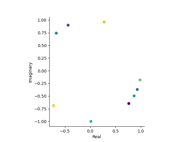
# Intro to complex numbers

def to_complex(x):
    return np.exp(1j*x)

def from_complex(x):
    x = np.angle(x)
    return np.where(x < 0, x + 2*np.pi, x)

# Let's plot the firs 10 trials in the complex plane
first_10_trials = experimental_paradigm.xs('attended', 0, 'condition')['x (radians)'].iloc[:10]

orientations_complex = to_complex(first_10_trials.values)

plt.figure()
plt.scatter(orientations_complex.real, orientations_complex.imag, c=first_10_trials.index)
plt.gca().set_aspect('equal')
plt.xlabel('Real')
plt.ylabel('Imaginary')
sns.despine()

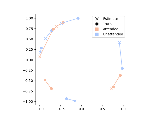
# Get posterior means by integrating over complex numbers
def wrap_angle(x):
    return np.mod(x + np.pi, 2*np.pi) - np.pi

def get_posterior_stats(posterior, ground_truth=None):
    posterior = posterior.copy()
    complex_grid = np.asarray(to_complex(posterior.columns))

    # Take integral over the posterior to get to the expectation (mean posterior)
    # In this case a complex number that we convert back to an angle between 0 and 2pi
    E = from_complex(np.trapezoid(posterior*complex_grid[np.newaxis,:], axis=1))

    # Take the integral over the posterior to get the expectation of the distance to the
    # mean posterior (i.e., standard deviation)
    relative_error = E[:, np.newaxis] - posterior.columns.values[np.newaxis,:]

    # Wrap the angle to be between 0 and pi, the error can never be larger than pi (180 degrees)
    relative_error = wrap_angle(relative_error)
    absolute_error = np.abs(relative_error)
    sd = np.trapezoid(absolute_error * posterior, posterior.columns, axis=1)

    stats = pd.DataFrame({'E':E, 'sd':sd}, index=posterior.index)

    if ground_truth is not None:
        stats['E_error'] = wrap_angle(stats['E'] - ground_truth)
        stats['E_error_abs'] = np.abs(stats['E_error'])
        stats['ground_truth'] = ground_truth

    return stats

posterior_stats = get_posterior_stats(conditional_orientation_ll, ground_truth=experimental_paradigm['x (radians)'].values)

# Circular correlations:
import pingouin as pg
posterior_stats.groupby('condition').apply(lambda d: pd.Series(pg.circ_corrcc(d['E'], d['ground_truth'], True), index=['rho', 'p']))

	rho	p
condition
attended	0.869551	1.522951e-13
unattended	0.372083	2.915933e-04

# Let's see how far the posterior mean is from the ground truth
# by plotting the estimates and groun truth in the complex plane
palette = sns.color_palette('coolwarm_r', 2)

# Create custom legend
legend_elements = [
    plt.Line2D([0], [0], marker='x', color='k', label='Estimate', markersize=8, linewidth=0),
    plt.Line2D([0], [0], marker='o', color='k', label='Truth', markersize=8, linewidth=0),
    plt.Line2D([0], [0], marker='s', color=palette[0], label='Attended', markersize=8, linewidth=0),
    plt.Line2D([0], [0], marker='s', color=palette[1], label='Unattended', markersize=8, linewidth=0)
]

# Plot the data
for ix, row in posterior_stats.iloc[:10].iterrows():
    hue = sns.color_palette('coolwarm_r', 2)[['attended', 'unattended'].index(ix[1])]

    estimate_complex = to_complex(row['E'])
    ground_truth_complex = to_complex(row['ground_truth'])

    plt.plot([estimate_complex.real, ground_truth_complex.real], [estimate_complex.imag, ground_truth_complex.imag], color=hue)
    plt.scatter(estimate_complex.real, estimate_complex.imag, color=hue, s=50, marker='x')
    plt.scatter(ground_truth_complex.real, ground_truth_complex.imag, color=hue, s=50, marker='o')

# Set aspect ratio and remove spines
plt.gca().set_aspect('equal')
sns.despine()

# Add legend
plt.legend(handles=legend_elements)

# Show the plot
plt.show()

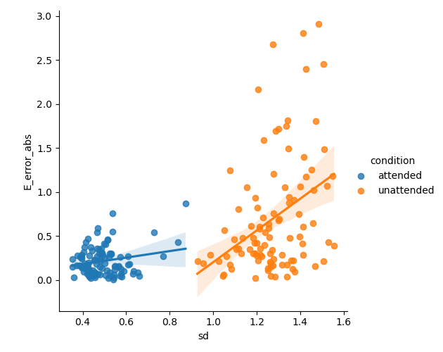
# Plot the error as a function of the standard deviation of the posterior
sns.lmplot(x='sd', y='E_error_abs', data=posterior_stats.reset_index(), hue='condition')

# %%

<seaborn.axisgrid.FacetGrid object at 0x17cd8aae0>