Expected decoding uncertainty via simulate + decode

Fisher information gives a local lower bound on the variance of any unbiased estimator of a stimulus from a fitted encoding model. It’s quick to compute and useful as a theoretical bound, but it ignores two things you usually care about in practice:

• the actual prior / stimulus distribution you’ll evaluate on,

• the bias of the maximum-a-posteriori or posterior-mean estimator (which Fisher info, being a Cramér–Rao bound, says nothing about).

A more direct alternative is to simulate from the fitted model and re-decode the simulated responses through the same model. The distribution of the posterior-mean estimate across many simulated trials at each stimulus value tells you:

• the bias \(E[\hat{s}] - s\), and

• the expected uncertainty \(\sqrt{\mathrm{Var}[\hat{s}]}\),

both as functions of the stimulus. This is the procedure used in neural_priors/encoding_model/get_expected_uncertainty.py; the example below ports it to public braincoder APIs on the bundled demo dataset.

import matplotlib.pyplot as plt
import numpy as np
import pandas as pd

from braincoder.models import LogGaussianPRF
from braincoder.optimize import ParameterFitter, ResidualFitter
from braincoder.utils.data import load_pratcarrabin2025_npc
from braincoder.utils.math import get_expected_value, get_sd_posterior
from braincoder.utils.stats import (
    fit_r2_mixture,
    get_rsq,
)

Load the demo + select voxels

Same voxel-selection step as the first two examples — kept self-contained.

bundle = load_pratcarrabin2025_npc()
r2 = bundle['r2']
paradigm_all = bundle['paradigm']
data_all = bundle['data']

r2_wb = bundle['r2_wholebrain'].get_fdata()
mask_wb = bundle['brain_mask'].get_fdata().astype(bool)
fit = fit_r2_mixture(r2_wb[mask_wb])
# Noise μ + 2σ on the logit scale — see example 1 for the rationale.
threshold = 1.0 / (1.0 + np.exp(-(fit['noise_mu'] + 2 * fit['noise_sigma'])))
keep = r2.index[r2 > threshold]
print(f'Kept {len(keep)} voxels (within-sample R² ≥ {threshold:.3f})')

# Restrict to wide-range trials and z-score within the selected voxel set.
is_wide = paradigm_all['range'].values == 'wide'
paradigm = paradigm_all.loc[is_wide].reset_index(drop=True)
data = data_all.loc[is_wide, keep].reset_index(drop=True).astype(np.float32)
data = (data - data.mean(axis=0)) / data.std(axis=0).replace(0, 1)
print(f'Data: {data.shape} (trials × voxels)')

Kept 155 voxels (within-sample R² ≥ 0.085)
Data: (240, 155) (trials × voxels)

Fit the encoding model on all trials

For an uncertainty estimate we want the model’s best guess at the true tuning curves — no held-out trials. The expected-uncertainty calculation only needs parameters and the noise model.

model = LogGaussianPRF(parameterisation='mu_sd_natural')
fitter = ParameterFitter(model, data, paradigm[['n']])

mu_grid   = np.linspace(10, 40, 16, dtype=np.float32)
sd_grid   = np.array([5., 10., 20.], dtype=np.float32)
amp_grid  = np.array([0.5, 1.0, 2.0], dtype=np.float32)
base_grid = np.array([0.0], dtype=np.float32)
init = fitter.fit_grid(mu_grid, sd_grid, amp_grid, base_grid)
pars = fitter.fit(max_n_iterations=600, init_pars=init,
                   noise_model='gaussian', learning_rate=0.05,
                   progressbar=False)

predictions = model.predict(paradigm=paradigm[['n']], parameters=pars)
predictions.index = data.index
train_r2 = get_rsq(data, predictions)
print(f'Train R² — median {np.nanmedian(train_r2):.3f}, '
      f'p90 {np.nanpercentile(train_r2, 90):.3f}')

Working with chunk size of 17921

  0%|          | 0/1 [00:00<?, ?it/s]
100%|██████████| 1/1 [00:00<00:00, 22.30it/s]
Number of problematic voxels (mask): 0
Number of voxels remaining (mask): 155
*** Fitting: ***
 * mu
 * sd
 * amplitude
 * baseline
Train R² — median 0.137, p90 0.198

Fit the noise model

Same Student-t noise model as notebook 2 (without geodesic regularisation here, to keep the example focused). init_pseudoWWT computes the W Wᵀ template over the stimulus grid we’ll later use for decoding.

stim_grid = pd.DataFrame({'n': np.arange(10, 41, 1, dtype=np.float32)})
stim_grid.index.name = 'stimulus'
model.init_pseudoWWT(stim_grid, pars)

resid_fitter = ResidualFitter(model, data, paradigm[['n']], parameters=pars)
omega, dof = resid_fitter.fit(method='t', init_dof=10.0,
                                max_n_iterations=600, progressbar=False)
print(f'Fitted dof: {dof:.1f}')

init_tau: 0.8408144116401672, 0.9756162762641907
USING A PSEUDO-WWT!
WWT max: 33.33961486816406
Fitted dof: 8.0

Simulate from the fitted model and re-decode

For every numerosity in the stimulus grid we draw n_repeats noise-perturbed response patterns, then push them through get_stimulus_pdf() to recover the posterior over numerosity. The posterior mean E is a per-trial estimate of the stimulus.

n_repeats = 200
print(f'Simulating {n_repeats} trials per numerosity '
      f'({len(stim_grid)} numerosities) …')
sim = model.simulate(paradigm=stim_grid, parameters=pars,
                      noise=omega, dof=dof, n_repeats=n_repeats)
print(f'Simulated data: {sim.shape}')

# Decode every simulated trial through the same model + noise.
posterior = model.get_stimulus_pdf(
    sim, parameters=pars, omega=omega, dof=dof,
    stimulus_range=stim_grid, normalize=True,
)

E = get_expected_value(posterior, normalize=True).to_frame('E_decoded')
E['true_n'] = np.tile(stim_grid['n'].values, n_repeats)
E['error']  = E['E_decoded'] - E['true_n']
sd_post = get_sd_posterior(posterior, E=E['E_decoded'].values, normalize=True)
E['posterior_sd'] = sd_post.values

Simulating 200 trials per numerosity (31 numerosities) …
Simulated data: (6200, 155)

Aggregate and plot

Per true numerosity, take the mean and standard deviation of the decoded \(\\hat{s}\) across simulated repeats — these are the bias and expected uncertainty curves.

summary = E.groupby('true_n').agg(
    mean_decoded=('E_decoded', 'mean'),
    std_decoded=('E_decoded', 'std'),
    mean_error=('error', 'mean'),
    mean_posterior_sd=('posterior_sd', 'mean'),
)
print(summary.round(3).head())

fig, axes = plt.subplots(1, 2, figsize=(11, 4.2))

ax = axes[0]
ax.plot(summary.index, summary['mean_decoded'], 'o-', color='#1f77b4',
         label='Mean decoded')
ax.fill_between(summary.index,
                 summary['mean_decoded'] - summary['std_decoded'],
                 summary['mean_decoded'] + summary['std_decoded'],
                 color='#1f77b4', alpha=0.2,
                 label='± std across repeats')
lim = (summary.index.min() - 1, summary.index.max() + 1)
ax.plot(lim, lim, 'k:', lw=1, label='Identity')
ax.set_xlim(lim); ax.set_ylim(lim)
ax.set_xlabel('True numerosity')
ax.set_ylabel(r'Decoded $\hat{n}$')
ax.set_title('Bias of posterior mean')
ax.legend(fontsize=8)

ax = axes[1]
ax.plot(summary.index, summary['std_decoded'], 'o-', color='#d62728',
         label='SD of decoded across repeats')
ax.plot(summary.index, summary['mean_posterior_sd'], 's--', color='#2ca02c',
         label='Mean posterior SD')
ax.set_xlabel('True numerosity')
ax.set_ylabel('Expected uncertainty')
ax.set_title('Decoding precision vs. stimulus')
ax.legend(fontsize=8)

fig.tight_layout()
plt.show()

        mean_decoded  std_decoded  mean_error  mean_posterior_sd
true_n
10.0       18.976000        5.974       8.976              7.748
11.0       19.596001        5.145       8.596              7.850
12.0       21.056000        4.870       9.056              7.994
13.0       21.833000        4.209       8.833              7.849
14.0       21.833000        3.833       7.833              7.564

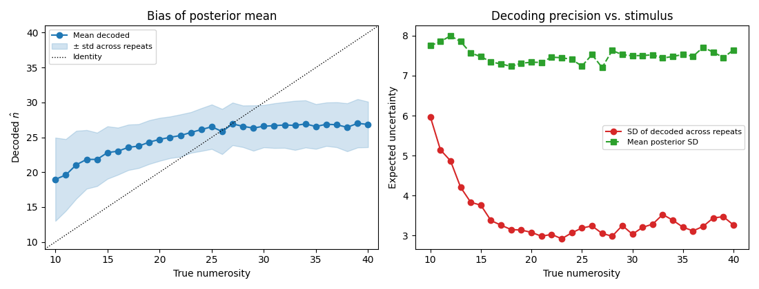
Interpretation

• The bias curve (left) shows whether the model systematically over- or under-estimates the true stimulus. A flat identity-line means no bias. Deviations often appear near the edges of the stimulus range (the encoding model can’t extrapolate beyond what it was fit on).

• The expected uncertainty curve (right) compares two flavours: the SD of the posterior mean across repeats (sampling uncertainty) and the mean posterior SD within a single decode (model-implied uncertainty). They tend to track each other but not match perfectly; large gaps point at mis-specification.

• Compared to Fisher information, this estimator captures realistic bias and prior effects at the cost of being slower (we have to simulate + decode \(\\sim 10^3\)–\(10^4\) trials).