Lesson 4: From neural responses to stimulus features#
Now we have a likelihood function \(p(x|s;\theta)\), we know, for a given stimulus, how likely different multivariate neural responses are. What we might be interested in the inverse, \(p(s|x;\theta)\), how likely different stimuli are for a given BOLD pattern.
To get here, we can use Bayes rule:
- Note that
We need to define a prior \(p(s)\)
To be able to integrate over \(p(s|x, \theta)\) we need to approximate \(p(x)\) by normalisation.
In practice, for simple one or two-dimensional stimulus space, we can use a uniform prior and evaluate likelihoods at a grid of useful points within that prior.
The crucial insight here is that we, for a given neural response pattern \(x\) try out which of a large set of possible stimuli are actually consistent with this neural response pattern
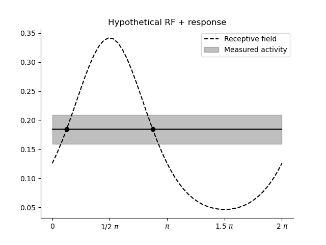
Let’s say we observed the following orientation receptive field, centered around a half \(pi\) and we observe, in unseen data, an activation of slightly less than 0.2:

We can now set up a likelihood function and find which stimuli are consistent with this activation pattern as follows.
First set up the model..
parameters = pd.DataFrame([{'mu':0.5*np.pi, 'kappa':1., 'amplitude':1.0, 'baseline':0.0}]).astype(np.float32)
weights = np.array([[1]]).astype(np.float32)

model = VonMisesPRF(parameters=parameters, weights=weights)
omega = np.array([[0.1]]).astype(np.float32)

data = pd.DataFrame([y]).astype(np.float32)
Then evaluate the likelihood for different orientations
orientations = np.linspace(0.0, 2*np.pi).astype(np.float32)
likelihood = model.likelihood(orientations, data, parameters, weights, omega)

# And plot it..
plt.figure()
plt.plot(orientations, likelihood.T, c='k')
plt.xticks([0.0, .5*np.pi, np.pi, 1.5*np.pi, 2*np.pi], ['0', '1/2 $\pi$', '$\pi$', '1.5 $\pi$', '2 $\pi$'])

sns.despine()
plt.xlabel('Orientation')
plt.ylabel('Likelihood')

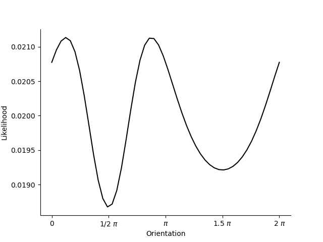
You can see that the likelihood is highest around \(\frac{1}{8}\pi\) and \(\frac{3}{8}\pi\)! With only one receptive field the predictions for these two points in stimulus space are identical!
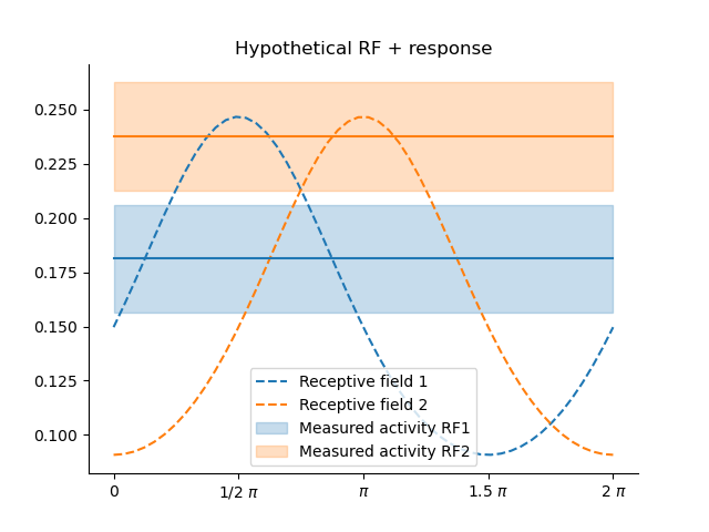
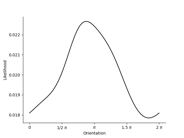
If we have two RFs, the situation becomes unambiguous:

parameters = pd.DataFrame([{'mu':0.5*np.pi, 'kappa':.5, 'amplitude':1.0, 'baseline':0.0},
                           {'mu':1.*np.pi, 'kappa':.5, 'amplitude':1.0, 'baseline':0.0}]).astype(np.float32)

model = VonMisesPRF(parameters=parameters)
omega = np.array([[0.05, 0.0], [0.0, 0.05]]).astype(np.float32)

dist1 = ss.vonmises(loc=.5*np.pi, kappa=.5)
dist2 = ss.vonmises(loc=1.*np.pi, kappa=.5)
x = 7./8.*np.pi
y1 =dist1.pdf(x)
y2 =dist2.pdf(x)

data = pd.DataFrame([[y1, y2]]).astype(np.float32)

likelihood = model.likelihood(orientations, data, parameters, None, omega)

plt.plot(orientations, likelihood.T, c='k')
plt.xticks([0.0, .5*np.pi, np.pi, 1.5*np.pi, 2*np.pi], ['0', '1/2 $\pi$', '$\pi$', '1.5 $\pi$', '2 $\pi$'])

sns.despine()
plt.xlabel('Orientation')
plt.ylabel('Likelihood')

Note
The complete Python script and its output can be found here.
Summary#
We have seen how to set up a simple encoding model and how to invert it to see which stimulis \(s\) are consistent with a given neural response \(x\).
For real data we of course have hundreds of voxels and thousands of stimuli. In the next tutorial we will see how we can decode data in a more natural setting.